Qini curves for uplift regression

This example demonstrates the use of Qini curves for uplift regression problems, where the target variable is continuous (e.g., spend amount instead of binary conversion).

The same Qini curve and uplift curve functions work for both classification and regression problems.

The idea of using Qini curves for continuous outcomes was discussed in: Nicholas J. Radcliffe, “Using Control Groups to Target on Predicted Lift: Building and Assessing Uplift Models”

The necessary imports

import numpy as np
np.random.seed(123)

import matplotlib.pyplot as plt

from sklearn.model_selection import train_test_split
from sklearn.preprocessing import OneHotEncoder
from sklearn.preprocessing import StandardScaler
from sklearn.compose import ColumnTransformer
from sklearn.linear_model import LinearRegression

from libuplift.meta import TLearnerUpliftRegressor
from libuplift.metrics import uplift_curve, Qini_curve
from libuplift.metrics import optimal_uplift_curve, optimal_Qini_curve
from libuplift.metrics import Qini_coefficient

Fetch and prepare data

from libuplift.datasets import fetch_Hillstrom
D = fetch_Hillstrom(as_frame=True)
trt = D.treatment

# encode categorical features, standardize numerical features
ct = ColumnTransformer([("ohe", OneHotEncoder(), list(D.categ_values.keys()))],
                       remainder=StandardScaler())
X = ct.fit_transform(D.data)

# keep only women's campaign
mask = ~(trt == 1)
X = X[mask]
y = D.target_spend[mask]
trt = (trt[mask] == 2)*1

Fit a model

X_train, X_test, y_train, y_test, trt_train, trt_test = train_test_split(X, y, trt, train_size=0.7)
m = TLearnerUpliftRegressor(base_estimator=LinearRegression())
m.fit(X_train, y_train, trt_train, n_trt=1)

TLearnerUpliftRegressor()

In a Jupyter environment, please rerun this cell to show the HTML representation or trust the notebook.
On GitHub, the HTML representation is unable to render, please try loading this page with nbviewer.org.

Draw Qini curves

score = m.predict(X_test)

cx, cy = Qini_curve(y_test, score, trt_test, n_trt=1)
cx_opt, cy_opt = optimal_Qini_curve(y_test, trt_test, n_trt=1)
plt.plot(cx, cy, label="curve")
plt.plot(cx_opt, cy_opt, "r-", label="optimal")
plt.plot([0,1], [0,cy[-1]], "k-", label="random")
plt.title("Qini curve (spend)")

plt.figlegend(ncols=3, loc="lower center")
plt.show()

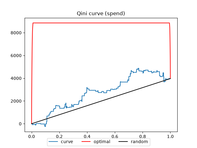
While Radcliffe et al. discourage using the optimal Qini curves for regression is discourages and another q_0 coefficient is suggested, libuplit allows for calculating optimal curves also for regression as shown above. The optimal curves are flat in the center due to many target values being exactly zero.

The Qini coefficient is also defined:

print("Qini coefficient = ", Qini_coefficient(y_test, score, trt_test, n_trt=1))

Qini coefficient =  0.10710744697449383

Uplift curves for regression problems

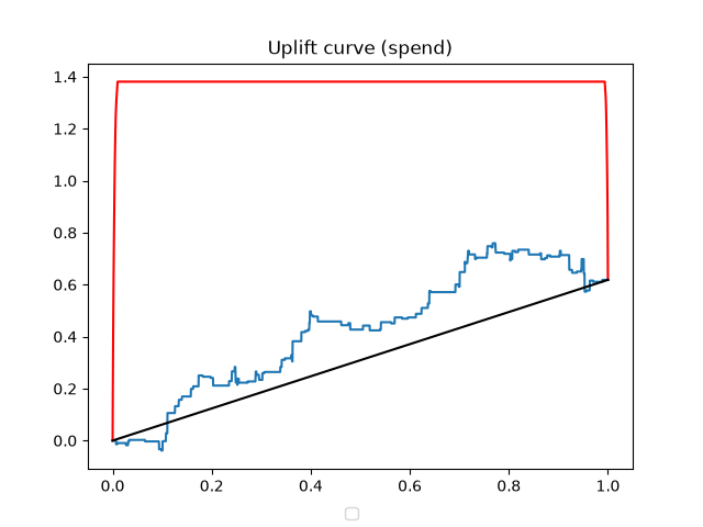
Uplift curves can also be used for regression problems. The y-axis now corresponds to average net gain in spend per customer.

cx, cy = uplift_curve(y_test, score, trt_test, n_trt=1)
cx_opt, cy_opt = optimal_uplift_curve(y_test, trt_test, n_trt=1)
plt.plot(cx, cy)
plt.plot(cx_opt, cy_opt, "r-")
plt.plot([0,1], [0,cy[-1]], "k-")
plt.title("Uplift curve (spend)")

plt.figlegend(ncols=3, loc="lower center")
plt.show()

/home/docs/checkouts/readthedocs.org/user_builds/libuplift/checkouts/latest/examples/evaluation/Qini_curves_for_uplift_regression.py:109: UserWarning: No artists with labels found to put in legend.  Note that artists whose label start with an underscore are ignored when legend() is called with no argument.
  plt.figlegend(ncols=3, loc="lower center")

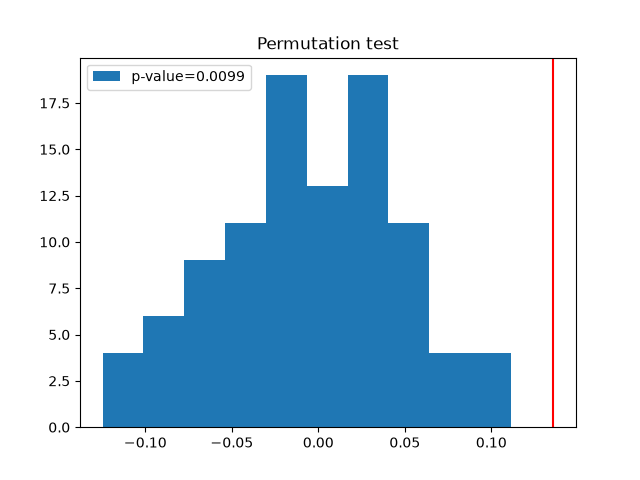
Evaluating model significance using a permutation test

from libuplift.model_selection import permutation_test_score

score, permutation_scores, pv =\
    permutation_test_score(m, X, y, trt, n_trt=1, cv=3,
                           n_permutations=100, scoring="Qini_coeff",
                           verbose=10, n_jobs=-1)
plt.hist(permutation_scores, density=False, label=f"p-value={pv:.4f}")
plt.axvline(score, color="r")
plt.title("Permutation test")
plt.legend()
plt.show()

[Parallel(n_jobs=-1)]: Using backend LokyBackend with 2 concurrent workers.
[Parallel(n_jobs=-1)]: Done   1 tasks      | elapsed:    0.1s
[Parallel(n_jobs=-1)]: Batch computation too fast (0.13320684432983398s.) Setting batch_size=2.
[Parallel(n_jobs=-1)]: Done   4 tasks      | elapsed:    0.3s
[Parallel(n_jobs=-1)]: Done  14 tasks      | elapsed:    0.8s
[Parallel(n_jobs=-1)]: Done  24 tasks      | elapsed:    1.2s
[Parallel(n_jobs=-1)]: Done  38 tasks      | elapsed:    1.9s
[Parallel(n_jobs=-1)]: Done  52 tasks      | elapsed:    2.5s
[Parallel(n_jobs=-1)]: Done  70 tasks      | elapsed:    3.4s
[Parallel(n_jobs=-1)]: Done  88 tasks      | elapsed:    4.2s
[Parallel(n_jobs=-1)]: Done 100 out of 100 | elapsed:    4.7s finished

We see that the model significantly outperforms random predictions.